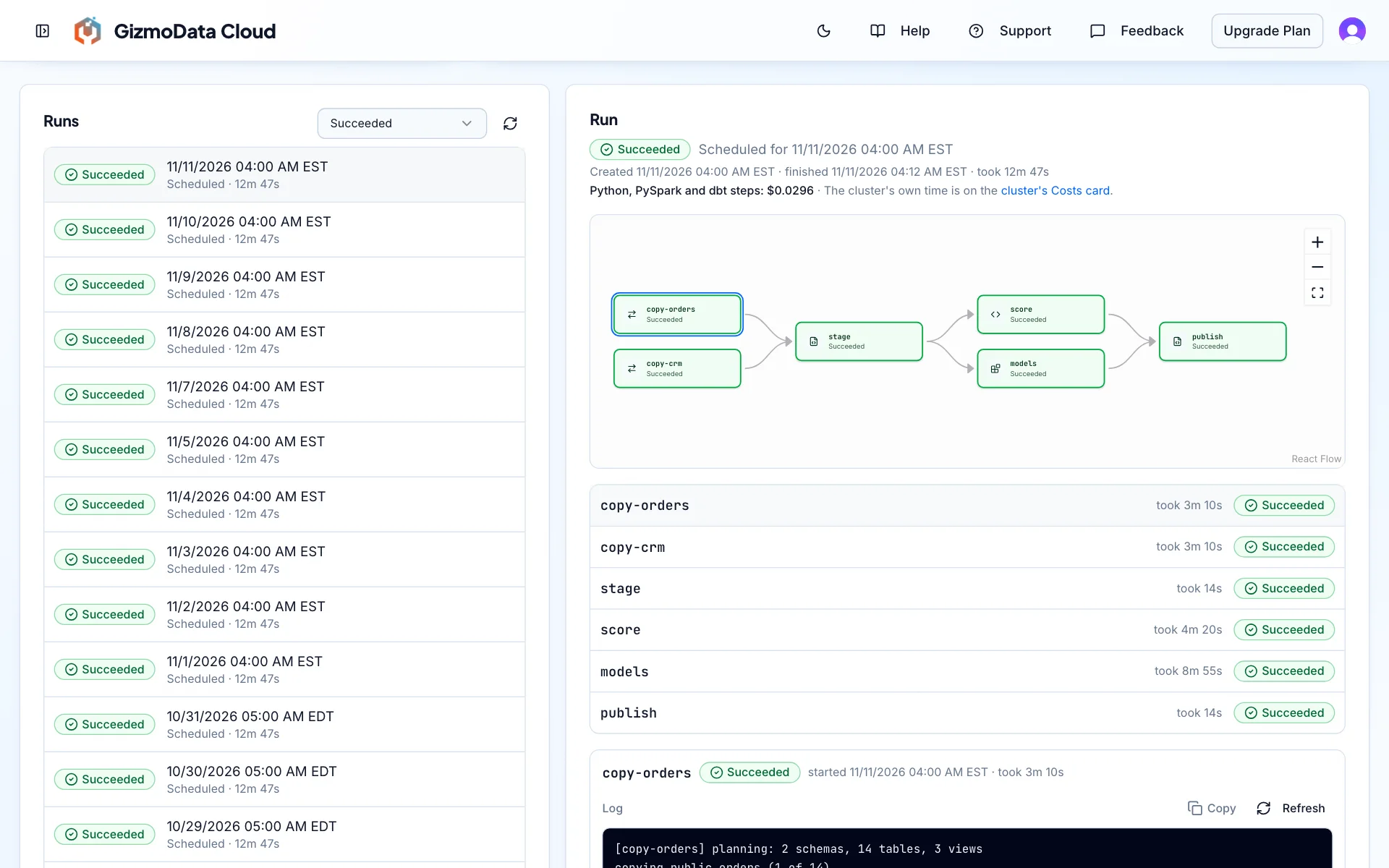
GizmoData Cloud now runs the work around your Hardcharger clusters: scheduled jobs that copy data in and run SQL, Python, PySpark and dbt, JupyterLab notebooks next to your data, and saved connections to the databases you already have. All of it is live today at app.gizmodata.com, and every run shows what its code steps cost.
Jobs with replication and SQL steps, connections and the rest of what follows work on AWS, Google Cloud and Azure. Python, PySpark and dbt steps and notebooks run where a data plane offers them: today that is AWS US East 2 (Ohio). These are Hardcharger features; GizmoSQL clusters keep working as before.
Schedule your pipelines
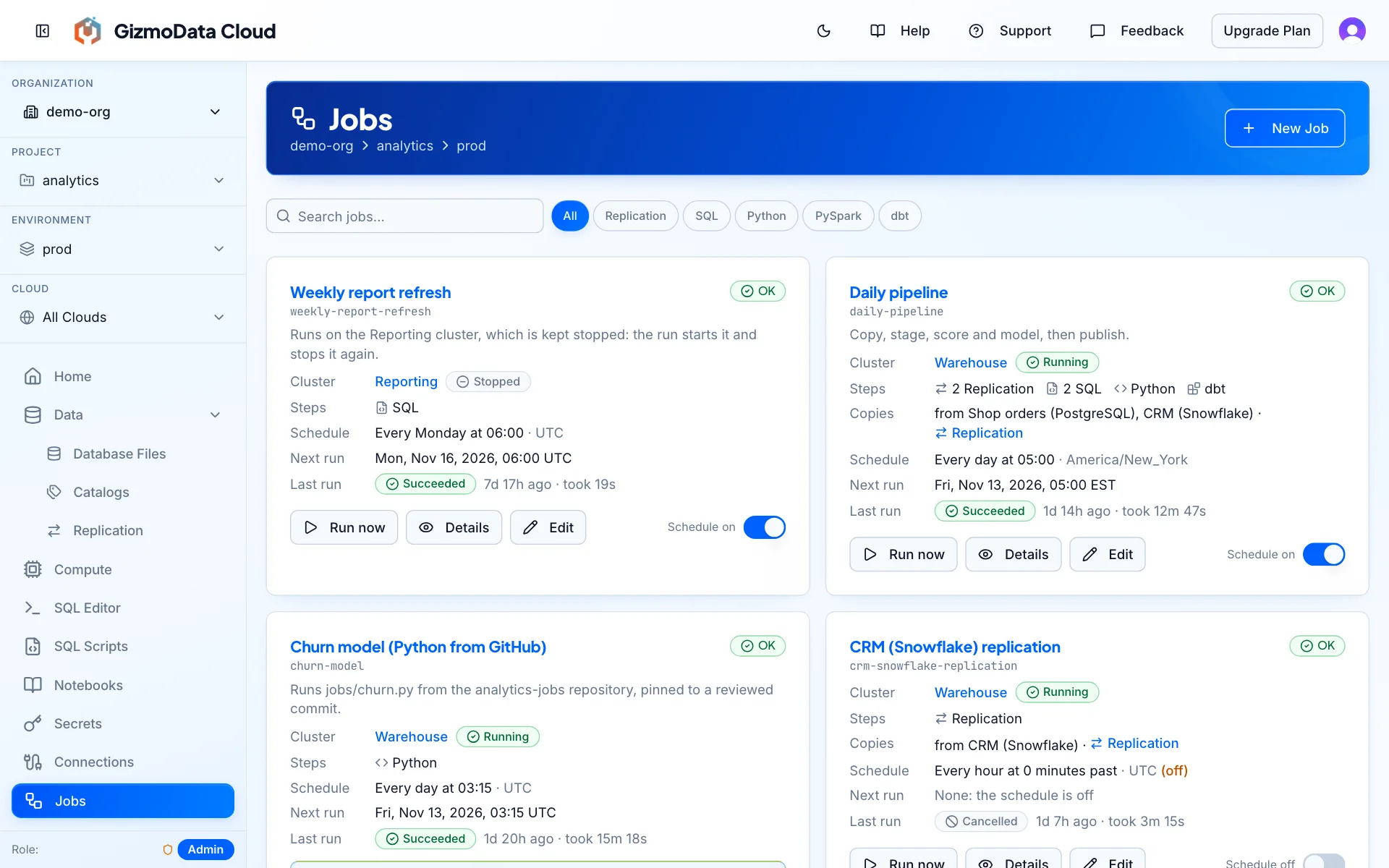
A job is a set of steps you draw as a graph on a Hardcharger cluster. Each step starts once the steps before it have succeeded, and steps that wait for nothing run side by side. There are five kinds of step: Replication, SQL, Python, PySpark and dbt. Run a job on a schedule, in the time zone you choose, or whenever you like with Run now.
Python and PySpark steps run your own code, typed in or fetched from a GitHub repository, with a connection to the cluster already signed in, so no password goes in the code. A dbt step runs a dbt Core project from a GitHub repository, and the platform writes the connection profile for you. Every run keeps its history and live logs, and your organization can get a Slack message when a job starts failing and when it works again. A run starts a cluster that stopped for being idle; with Start the cluster if it is stopped switched on, it also starts a cluster a person stopped, and stops it again when the run ends. Your code runs on machines of its own, apart from other organizations.
Keep data in sync
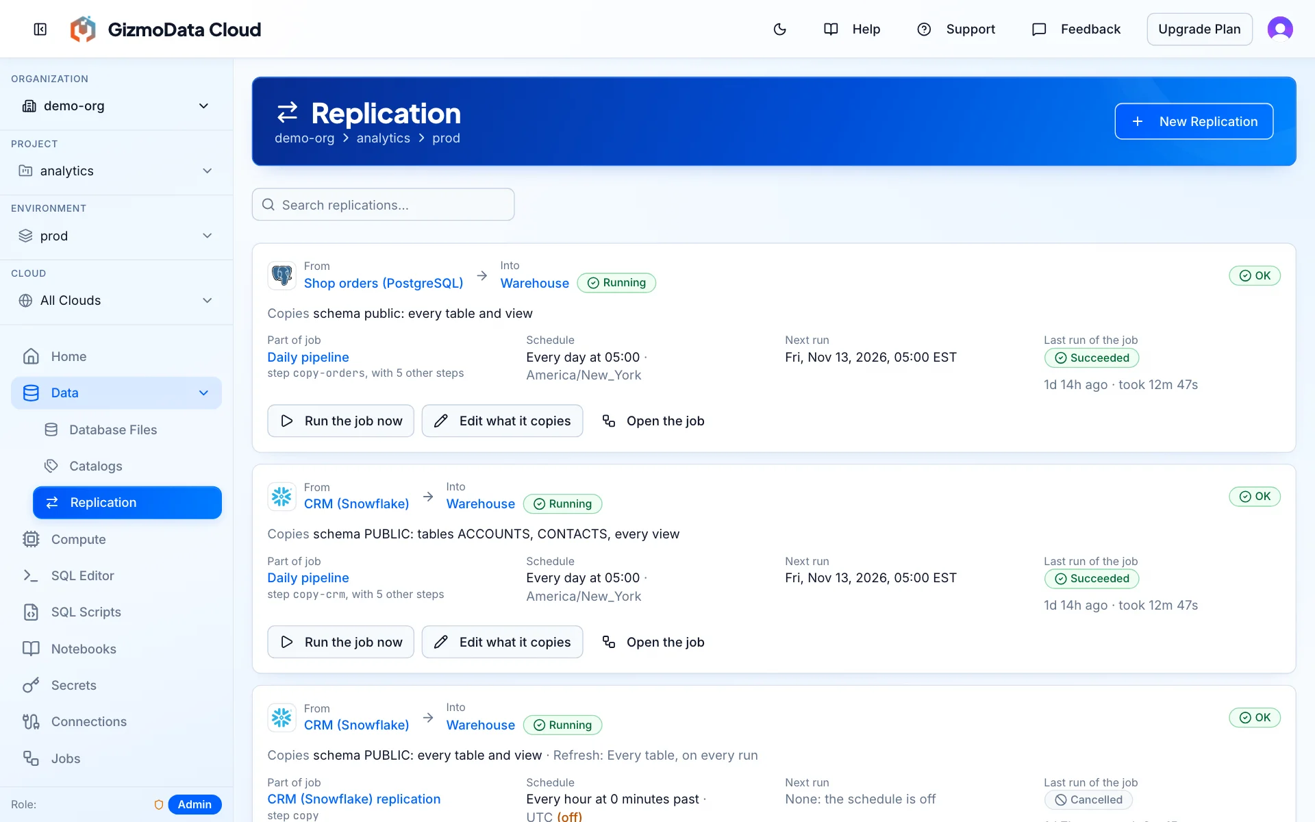
Replication copies tables and views into a Hardcharger cluster from PostgreSQL, Oracle Database, Snowflake or another Hardcharger server, and keeps the copy up to date on a schedule. Choose schemas, tables and views by pattern, and Plan shows what a run would copy before anything is copied. Leave columns out, or mask them with a SHA-256 hash or an empty value: masks run in the source database, so the real values never leave it. Views are recreated on the cluster, with their SQL translated for it.
Each replication is a step of a job, so SQL or dbt steps can run right after the copy. The new Data > Replication page lists every replication with its source, its cluster, its schedule and how its last run went.
Work in notebooks next to your data
Start a JupyterLab session next to a Hardcharger cluster and it opens in a new tab, already signed in to the cluster as you, with your own access to it. It has a Python and a PySpark kernel (PySpark DataFrame operations run on the cluster itself, with no Spark cluster to start), %%sql cells and Git. Your notebooks, data and the Python packages you install stay in a workspace on the cluster for your next session, and JupyterLab carries GizmoData Cloud’s colours and logo, so a notebook tab is easy to tell apart.
A new workspace starts with an Examples folder: a Python quickstart and a PySpark quickstart. This is the first query of the Python quickstart, where conn is a connection to your cluster that is already there:
1# Run a query on the cluster and show its rows as a table.
2# Expect five rows: the numbers 1 to 5 and their squares.
3# This is the first statement, so the connection opens here: it can take a few seconds.
4with conn.cursor() as cursor:  # "with" closes the cursor at the end of the block
5    cursor.execute(operation="SELECT range AS n, range * range AS square FROM range(1, 6)")
6    squares = cursor.fetch_arrow_table()  # the rows as an Arrow table: columns with their types
7
8squares.to_pandas()  # the same rows as a pandas DataFrame, shown below the cell
And the same kind of query in a %%sql cell, which runs on the same connection and shows its result as a table:
%%sql
-- Everything in this cell is SQL, sent to the cluster as written.
-- Several statements may be separated by ";": they run in turn, and the last one's
-- result is shown as a table (a pandas DataFrame).
-- Expect one row: the number of rows and the sum of the squares from 1 to 5 (55).
SELECT count(*) AS numbers, sum(range * range) AS sum_of_squares
FROM range(1, 6)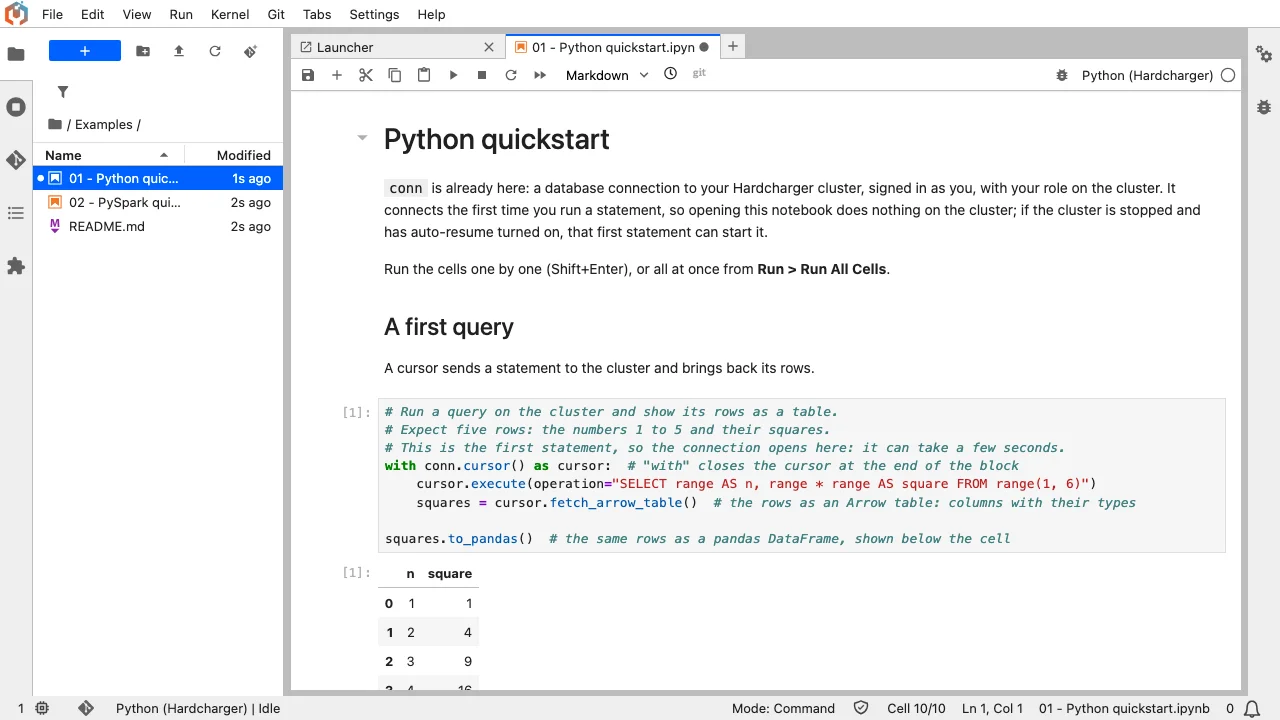
Connect what you already have
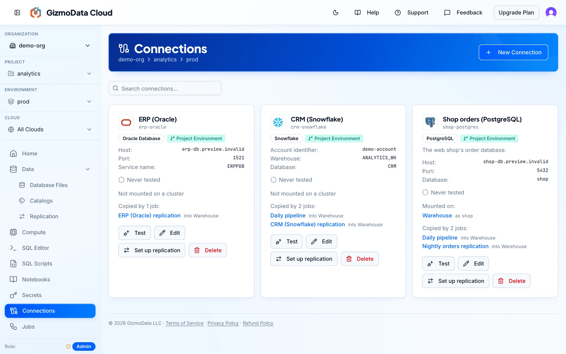
The new Connections page saves a connection to PostgreSQL, Snowflake, Oracle Database, IBM Db2, Quack, Hardcharger or GizmoSQL once. Test it from your data plane, then mount it on Hardcharger clusters and query its tables with SQL, next to your own data. The same connection can be the source of a replication: Set up replication starts one from its card.
Data in Amazon S3 needs no keys either. An AWS role secret lets a Hardcharger cluster read your S3 buckets through an IAM role in your own AWS account. No access key is stored, and short-lived credentials renew automatically.
See what it costs
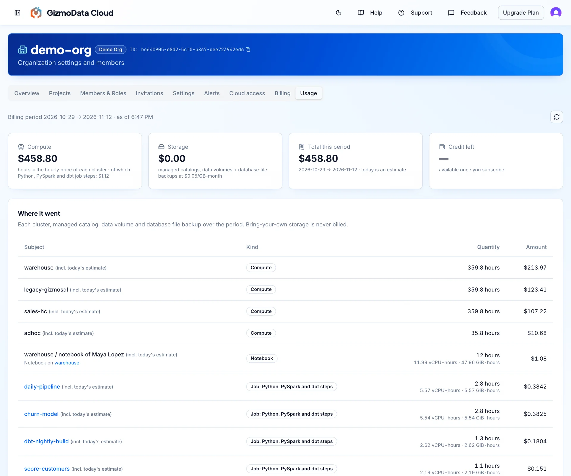
Python, PySpark and dbt steps and notebook sessions are billed for the time they run, by the second, at $0.062 per vCPU-hour plus $0.007 per GiB-hour of the size you choose. Replication and SQL steps have no charge of their own: the cluster’s running time is billed as before.
A step’s form and the notebook dialog show the price of the size you pick before you start. A run’s page shows what each Python, PySpark and dbt step used and what it came to, a job’s page shows its last 30 days, day by day, and Organization > Usage has a line for each job with Python, PySpark or dbt steps and for each notebook session, next to your clusters.
Also new: Catalogs, Compute, Connections, Jobs, Replication and the portal’s other lists have a search box that filters as you type, and after an update the portal shows what changed since your last visit. Help > What’s new lists every release.
Try it
Sign up, create a Hardcharger cluster, and open Jobs, Notebooks or Connections in the portal. The GizmoData Cloud page walks through each feature and lists the prices. We’d love to hear what you run on it: join the GizmoData Community Slack or get in touch.
Scheduled jobs, notebooks and connections are live on GizmoData Cloud.